TransformerVAE

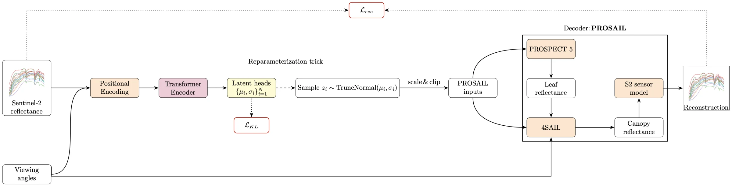
The Transformer–PROSAIL VAE is a physics-informed machine-learning system I built for retrieving vegetation biophysical parameters from Sentinel-2 imagery. It learns the inverse mapping from multispectral reflectance to physically meaningful variables while using the PROSAIL radiative-transfer model as a fixed decoder.

This design combines the representation capacity of a transformer with a scientific model that already encodes how leaf chemistry, canopy structure, soil, illumination, and viewing geometry produce a spectral signal. Instead of training a network to emit unconstrained labels, the model must infer parameters capable of reconstructing the observed reflectance through known physics.

The scientific problem

Satellite reflectance inversion is ill-posed: many combinations of leaf area, pigment concentration, canopy geometry, soil properties, atmosphere, and acquisition angle can produce similar spectra. A standard supervised regressor can fit a dataset while violating the forward process that produced the observation, and a point estimate hides ambiguity that matters to downstream environmental decisions.

PROSAIL provides the forward direction. It combines the PROSPECT leaf optical model with the 4SAIL canopy model to simulate spectral reflectance from biophysical variables and viewing geometry. The difficult task is the inverse: given a small set of Sentinel-2 bands, estimate a plausible distribution over those hidden variables.

I framed that inverse as a variational model. A transformer reads the spectral sequence, predicts parameters of bounded latent distributions, samples them with a differentiable reparameterization, maps them into physical PROSAIL ranges, and reconstructs the original observation through the fixed simulator and sensor response.

Model architecture

Spectral tokens and self-attention

The encoder treats each selected reflectance band and derived spectral index as a token. A learned linear projection moves scalar observations into a shared embedding space, learned positional embeddings retain band identity, and stacked multi-head self-attention models interactions across the spectrum.

The default transformer configuration uses a 64-dimensional embedding, four attention heads, two encoder layers, a four-times wider feed-forward block, dropout, and mean pooling across tokens. The pooled representation is projected into two parameters for each physical latent variable.

x_emb = self.token_embedding(encoder_input.unsqueeze(-1))
x_emb = x_emb + self.pos_embedding(positions)
 
encoded_seq = self.transformer_encoder(x_emb)
pooled = encoded_seq.mean(dim=1)
latent_out = self.linear_out(pooled)
 
dist_params = self.lat_space.get_params_from_encoder(latent_out)
z = self.sample_latent_from_params(dist_params, n_samples=n_samples)
sim = self.transfer_latent(z)
reconstruction = self.decode(sim, angles)

The transformer posterior currently uses spectral bands and optional indices as its token sequence. Acquisition angles are carried separately into the PROSAIL decoder, where they condition the reconstruction. Making viewing geometry a first-class encoder token is a clear extension point in the implementation.

Bounded probabilistic latent space

Each encoder head defines the location and scale of a truncated normal distribution on [0, 1]. Reparameterized sampling keeps the path differentiable, while the simulator-space transform scales normalized samples into physically meaningful parameter bounds.

The latent variables represent leaf structure, chlorophyll and carotenoid content, brown pigment, equivalent water thickness, dry matter, leaf area index, leaf-angle distribution, hotspot behavior, and soil terms. The code supports legacy and literature-updated priors, Gaussian or uniform sampling laws, LAI-correlated parameter generation, disabled variables for controlled experiments, and KL divergence against bounded priors.

Physics as the decoder

The decoder contains no learned replacement for radiative transfer. It concatenates sampled physical variables with illumination and viewing angles, runs PROSAIL, then integrates the high-resolution output through a sensor response simulator to reconstruct the selected satellite bands.

This creates an interpretable training signal: a latent estimate is useful only when the corresponding physical simulation explains the measured spectrum. The sensor layer supports Sentinel-2 and EnMAP and includes a generic spectral-response implementation for testing additional instruments.

Multi-objective training

The training system combines reconstruction likelihood with latent KL regularization and optional supervision, spectral-index, and cyclical consistency terms. It supports diagonal, full, hybrid, and mean-squared reconstruction losses, Monte Carlo samples, gradient accumulation, exponential or plateau learning-rate scheduling, and switching from hybrid to full likelihood late in training.

To reduce sensitivity to poor initialization, the pipeline can train multiple candidate models briefly, compare validation reconstruction loss, and keep the best starting point. It records training and validation curves, memory use, learning-rate history, gradient flow, checkpoint state, and optional CodeCarbon emissions telemetry.

Synthetic dataset engineering

The repository includes an end-to-end generator for the inverse problem's training data:

1. Sample valid PROSAIL variables from configurable physical distributions.
2. Optionally correlate chlorophyll, leaf structure, water, dry matter, and canopy variables with LAI.
3. Sample solar zenith, view zenith, and relative azimuth angles.
4. Run simulations in bounded batches to control memory.
5. Convolve spectra with Sentinel-2 or EnMAP response functions.
6. Save reflectance, physical variables, viewing geometry, and normalization coefficients as tensor artifacts.

The standard workflow produces 500,000 training examples and separate 10,000-example validation and test sets. Normalization can use mean-scale or robust quantile factors, and the loaders support deterministic subsets, train/validation splits, k-fold experiments, image patches, and MMDC Earth-observation datasets.

Inference and uncertainty

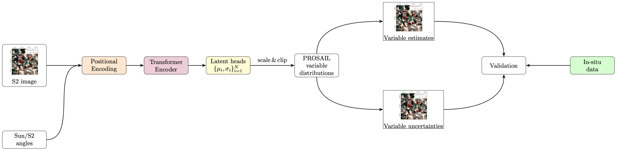
At inference time the model can return the latent mode, truncated-Gaussian expectation, simulator-space mode, median, expectation, or Monte Carlo samples. Those alternatives matter because the nonlinear transform from normalized latent space into PROSAIL variables means the mean before transformation is not always the mean after it.

The output includes both parameter estimates and uncertainty. Reconstructed spectra provide an additional diagnostic: large spectral residuals can identify observations that are poorly explained by the learned posterior or the assumptions of the forward model.

The implementation handles individual spectra and spatial image patches. Utilities flatten patches for model execution and restore spatial dimensions afterward, allowing parameter and uncertainty maps to be written back into georeferenced raster products.

Field validation

I built a geospatial validation pipeline around two independent field-data programs:

• BelSAR 2018 agricultural measurements in Belgium, including maize and wheat campaigns across multiple Sentinel-2 acquisitions
• FRM4VEG observations from Barrax in 2018 and 2021 and Wytham in 2018, spanning crops, bare soil, and deciduous forest

The workflow reads Sentinel-2 products, harmonizes coordinate systems, builds field-plot windows, extracts reflectance and acquisition geometry, aligns observations in space and time, interpolates predictions when field dates fall between acquisitions, and compares the posterior estimates with in-situ Leaf Area Index (LAI) and Canopy Chlorophyll Content (CCC).

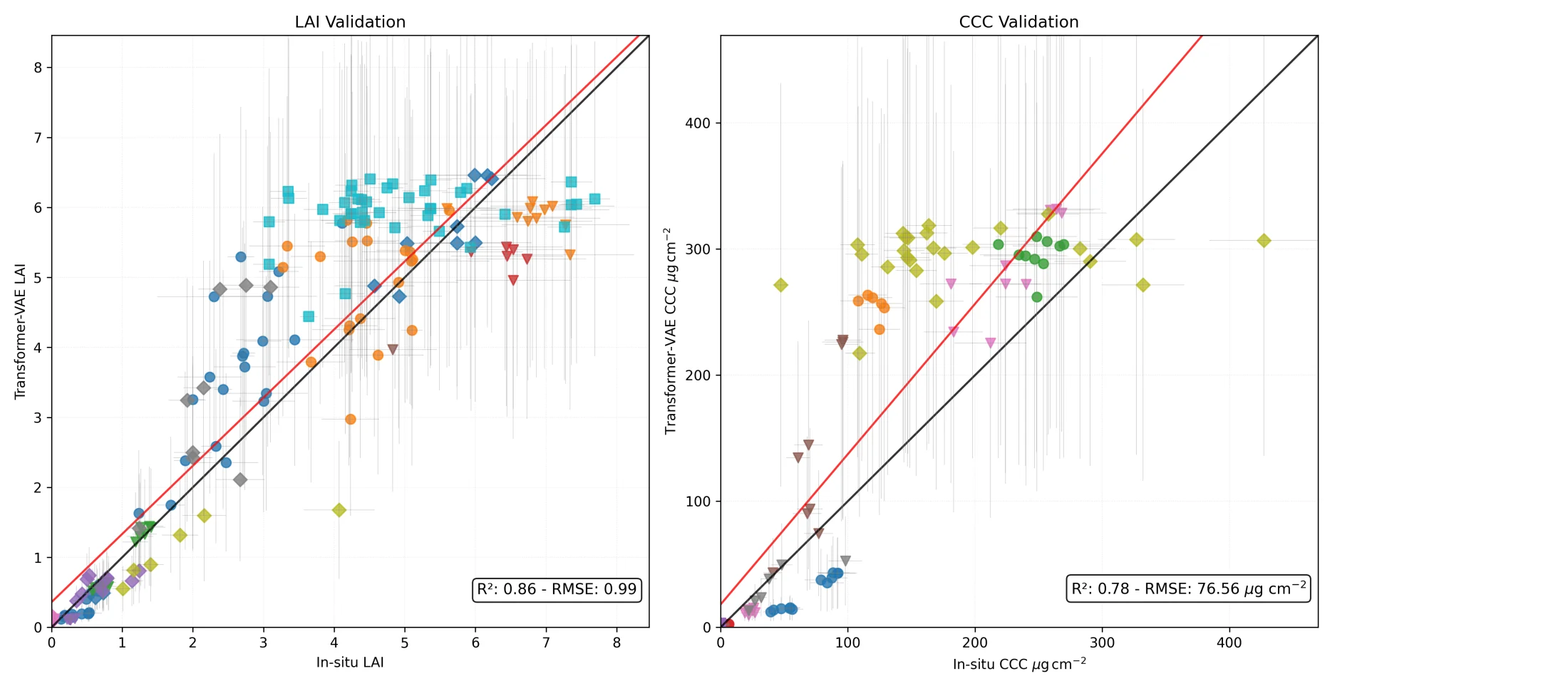
Across the combined validation artifacts, LAI achieves an RMSE of 0.99. The repository's alternative aggregation figures report LAI R² values between 0.83 and 0.86, while the documented all-site summary reports 0.85. Site-level LAI RMSE is 0.63 at Barrax 2021, 0.72 at Barrax 2018, 1.03 for BelSAR, and 1.53 at Wytham.

The CCC result has an all-site RMSE of 76.56 µg cm⁻² and visibly wider intervals. I present that honestly: the model captures substantial structure, but chlorophyll generalization and uncertainty calibration remain weaker than LAI, especially across heterogeneous vegetation and field protocols.

The evaluation package computes RMSE, R², mean absolute and relative error, Mean Prediction Interval Width, and Prediction Interval Coverage Probability. Detailed CSV outputs preserve each observation, site, land cover, posterior standard deviation, temporal offset, reconstruction error, and per-band error for later analysis.

Engineering the research system

The project is implemented in PyTorch with NumPy, pandas, SciPy, scikit-learn, Rasterio, GeoPandas, Matplotlib, and domain-specific PROSAIL and Earth-observation libraries. Pixi defines a CUDA 11.8 research environment alongside a conventional requirements file, while shell entry points make dataset generation, transformer training, and multi-dataset validation repeatable.

The repository contains 36 Python modules, a 61 MB trained checkpoint archive, generated simulation tensors, georeferenced prediction rasters, 24 tracked figures, and detailed field-validation tables. Twelve test functions cover spectral response reading, generic sensor simulation, PROSAIL decoding, model construction, differentiable forward passes, distribution statistics, KL computation, regression behavior, and a one-epoch training pipeline.

I keep several limitations visible in the code and documentation:

• The current research environment relies on specialized Git-hosted scientific packages and GPU-oriented dependencies.
• Some validation commands retain machine-specific fallback paths that should become a single portable dataset registry.
• Reproducible release configuration and automated continuous integration need hardening before external benchmark claims.
• Field generalization and posterior calibration, particularly for CCC and forest observations, remain research questions rather than solved product features.

What this project demonstrates

This project demonstrates how I work at the boundary between machine learning and scientific software. It required translating radiative-transfer constraints into differentiable architecture, designing synthetic experiments, implementing probabilistic inference, handling satellite rasters and field geometries, and evaluating both accuracy and uncertainty.

It also reflects an engineering principle I value: use domain knowledge to reduce what the model is allowed to invent. The transformer learns the difficult inverse mapping, but the decoder remains anchored to physical process. That division makes the system more interpretable, diagnosable, and scientifically useful than an unconstrained black-box regressor.

If you are working on Earth observation, physics-informed learning, probabilistic inversion, or scientific ML infrastructure, review the repository or reach out by email.